Welcome to part 1 of our blog series on "Running Time Series Models in Production using CrateDB".
Introduction to Time Series Modeling
In this blog post, we will introduce you to the concept of time series modeling, and discuss the main obstacles faced during its implementation in production. We will then introduce you to CrateDB, highlighting its key features and benefits, why it stands out in managing time series data, and why it is an especially good fit for supporting machine learning models in production.
Whether you are a data scientist aiming to simplify your model deployment, a data engineer looking to enhance your data landscape, or a tech enthusiast keen on understanding the latest trends, this blog post will offer valuable insights and practical knowledge.
For readers familiar with data modeling, it is important to distinguish that time series modeling is a different discipline.
Main Time Series Modeling Techniques
Time series modeling is a crucial technique used across various sectors. Two main modeling techniques comprise the field of machine learning: Time series forecasting and anomaly detection.
Time Series Forecasting
Time series forecasting has applications in predicting future sales in retail, anticipating stock market trends in finance, predictive maintenance in manufacturing, user churn and subscription analysis in web applications, forecasting energy demand in utilities, and many others. It involves the use of statistical models to predict future values based on previously observed data.
Anomaly Detection
Anomaly detection is used to identify outliers or unusual patterns in time series data. This detection technique uses statistical and machine learning algorithms to sift through large data sets over specific time intervals, analyzing patterns, trends, cycles, or seasonality, to spot deviations from the norm. These anomalies could either be an error or indicate another kind of significant event you would like to be alerted about.
Anomaly detection is widely used in multiple fields and industries, including cybersecurity, where it identifies unusual network activity patterns that could signify a potential breach, in finance for spotting fraudulent activities in credit card transactions; and in IoT for detecting malfunctioning sensors and machines. Other use cases include healthcare, for monitoring unusual patient vital signs, and predictive maintenance, where it is used to identify abnormal machine behavior, in order to prevent system failures.
CrateDB: the perfect fit for time series data
While creating these models in itself is a challenging task, deploying them to production environments in a robust manner, is often equally challenging. More often than not, you will need to deal with large volumes of data, ensure real-time processing, manage and update feature stores, keep track of data and model versions, all while maintaining data accuracy and integrity.
This is where CrateDB comes into play. CrateDB is a distributed SQL database, designed specifically to handle the unique demands of time series data. It offers scalability, real-time data processing, and ease of use, making it an ideal choice for deploying time series and anomaly detection models. On top of that, CrateDB offers first-class analytical SQL support for time series data and binary blob data types, which makes it possible to store and retrieve machine learning models without needing extra infrastructure.
CrateDB is well integrated with the modern data processing and machine learning ecosystem through both its SQLAlchemy dialect and its PostgreSQL wire-protocol compatibility. It provides support and adapters for Apache Flink, Apache Kafka, Apache Spark, pandas, Dask, as well as Apache Superset, Tableau, and many more.
Time Series Prediction
Time series modeling is a statistical technique that utilizes sequential data to predict future values or events based on historical data. It involves analyzing patterns, trends, and seasonality in past data, to forecast future events. This type of forecasting is particularly useful when dealing with data that changes over time, such as stock prices, weather patterns, marketing & sales data, or M2M/IoT data.
Time series trend, seasonality and cyclicality
One of the key components of time series modeling is the understanding and interpretation of certain critical properties intrinsic to time series data, such as trend, seasonality, and cyclicality.
- Trend refers to the overall pattern or direction in which data is moving over a significant period.
- Seasonality are the recurring patterns or cycles that are typically observed within a specific time frame, be it daily, weekly, annually, etc.
- Cyclicality involves fluctuations that occur at irregular intervals, and cannot be linked to any particular season or event.
Applications
The ability to accurately predict future events based on past data is invaluable in many sectors. For instance, online shops can forecast product demand to manage inventory, financial institutions can predict stock prices to make informed investment decisions, and manufacturing companies can anticipate machine maintenance downtimes to efficiently plan their production schedules. By making accurate predictions, businesses can make predictive, data-based decisions, reduce risks, and improve efficiency.
Furthermore, time series modeling is also useful for anomaly detection. Anomalies are data points that deviate from the expected pattern or trend. They can be caused by a variety of factors, such as human error, equipment malfunction, or cyber-attacks. By detecting anomalies early on, businesses can take corrective actions to prevent further damage. For instance, a manufacturing company can detect anomalies in their production process to prevent machine breakdowns and avoid costly downtimes.
Time Series Analysis Models
Various types of models are employed in time series analysis, each with its strengths and weaknesses.
The simplest model is the autoregressive (AR) model, which assumes future values can be forecasted from a weighted sum of the past.
The moving average (MA) model, on the other hand, assumes that future values are a function of the mean and various random error terms.
More complex models, like autoregressive integrated moving average (ARIMA) and seasonal ARIMA (SARIMA), combine strategies from AR and MA models while also accounting for trends and seasonality.
Additionally, state-of-the-art models like Long Short-Term Memory (LSTM), a type of recurrent neural network, are effective at capturing long-term dependencies in time series data.
More recent models for anomaly detection are Random Cut Forest (RCF), Variational Auto Encoders (VAE), which are both neural network-based, unsupervised learning algorithms (with VAEs surprisingly being also very good in semi-supervised and supervised learning applications).
Honorable mentions in the field of time series anomaly detection are also the Isolation Forest (IF), One-Class Support Vector Machine (OCSVM) models, and the excellent prophet time series analysis library released by Facebook.
Furthermore, recent developments advise to not only use a single model for time series forecasting and anomaly detection, but multiple ones, called an ensemble. This technique uses multiple of the aforementioned models on the same data, and then combines their predictions to get a more accurate result. To get a practical hang of how time series modeling works, the next section will exercise a basic example.
Example: Times Series Anomaly Detection for Machine Data
Prologue
NOTE: While this example should provide more depth to understanding time series modeling, it is not intended to teach the foundations of this field of data science. Instead, it will focus more on how to use machine learning models in production scenarios. However, if you are interested in learning more about time series modeling, we recommend to check out Time Series Analysis in Python – A Comprehensive Guide with Examples, by Selva Prabhakaran.
About
The exercise will use the Numenta Anomaly Benchmark (NAB) dataset, which includes real-world and artificial time series data for anomaly detection research. We will choose the dataset about real measured temperature readings from a machine room.
The goal is to detect anomalies in the temperature readings, which could indicate a malfunctioning machine. The dataset simulates machine temperature measurements, and will be loaded into CrateDB upfront.
Setup
To follow this tutorial, install the prerequisites by running the following commands in your terminal. Furthermore, load the designated dataset into your CrateDB Cloud cluster.
Please note the following external dependencies of the merlion library:
OpenMP
Some forecasting models depend on OpenMP. Please install it before installing this package, in order to ensure that OpenMP is configured to work with the lightgbm package, one of Merlion's dependencies.
When using Anaconda, please run
When using macOS, please install the Homebrew package manager and invoke
Java
Some anomaly detection models depend on the Java Development Kit (JDK). On Debian or Ubuntu, run
On macOS, install Homebrew, and invoke
Also, ensure that Java can be found on your PATH, and that the JAVA_HOME environment variable is configured correctly.
Importing Time Series Data
If you are using CrateDB Cloud, navigate to the Cloud Console, and use the Data Import feature to import the CSV file directly from the given URL into the database table machine_data.
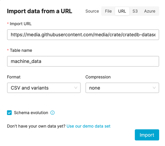
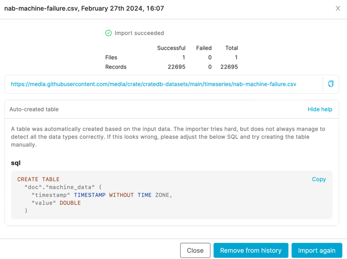
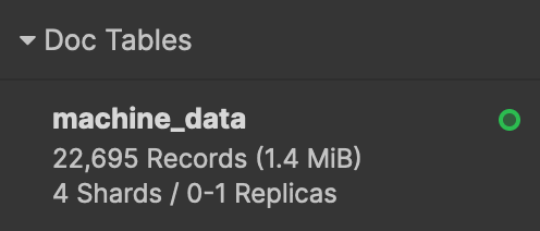
The import process will automatically infer an SQL DDL schema from the shape of the data source. When visiting the CrateDB Admin UI after the import process has concluded, you can observe the machine_data table was created and populated correctly.
If you want to exercise the data import on your workstation, use the crash command-line program.
Note: If you are connecting to CrateDB Cloud, use the options --hosts 'https://<hostname>:4200' --username '<username>'. In order to run the program non-interactively, without being prompted for a password, use export CRATEPW='<password>'.
Loading Time Series Data
First, you will load the dataset into a pandas DataFrame and convert the timestamp column to a Python datetime object.
Downsampling Time Series Data
TIP: CrateDB provides many useful analytical functions tailored for time series data. One of them is the date_bin which bins the input timestamp to the specified interval - which makes it very handy to resample data.
In general, for time series modeling, you often want to sample your data with a high frequency, in order not to miss any events. However, this results in huge data volumes, increasing the costs of model training. Here, it is best practice to down-sample your data to reasonable intervals.
This SQL statement demonstrates CrateDB's date_bin function to down-sample the data to 5-minute intervals, reducing both the amount of data and the complexity of the modeling process.
Plotting Time Series Data
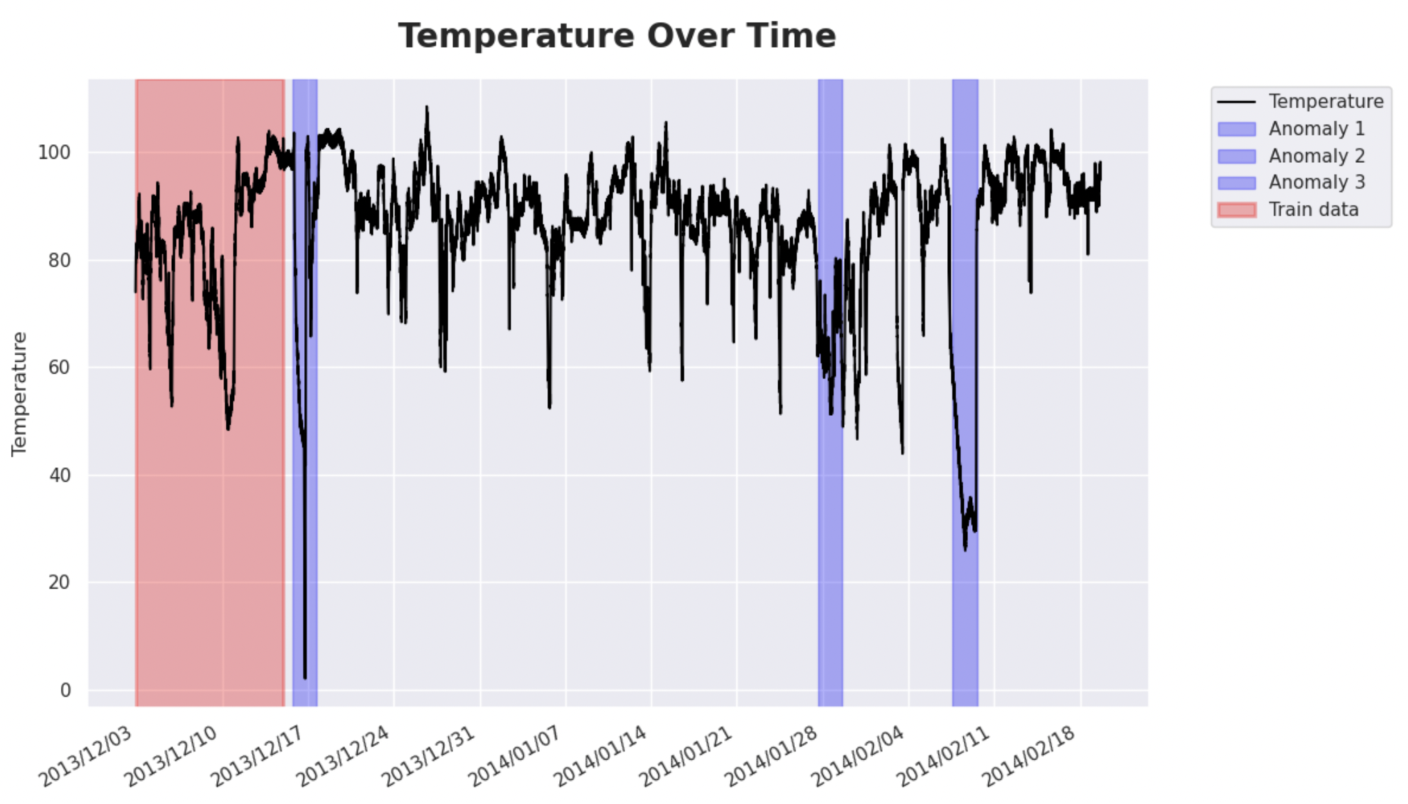
Next, plot the data to get a better understanding of the dataset.
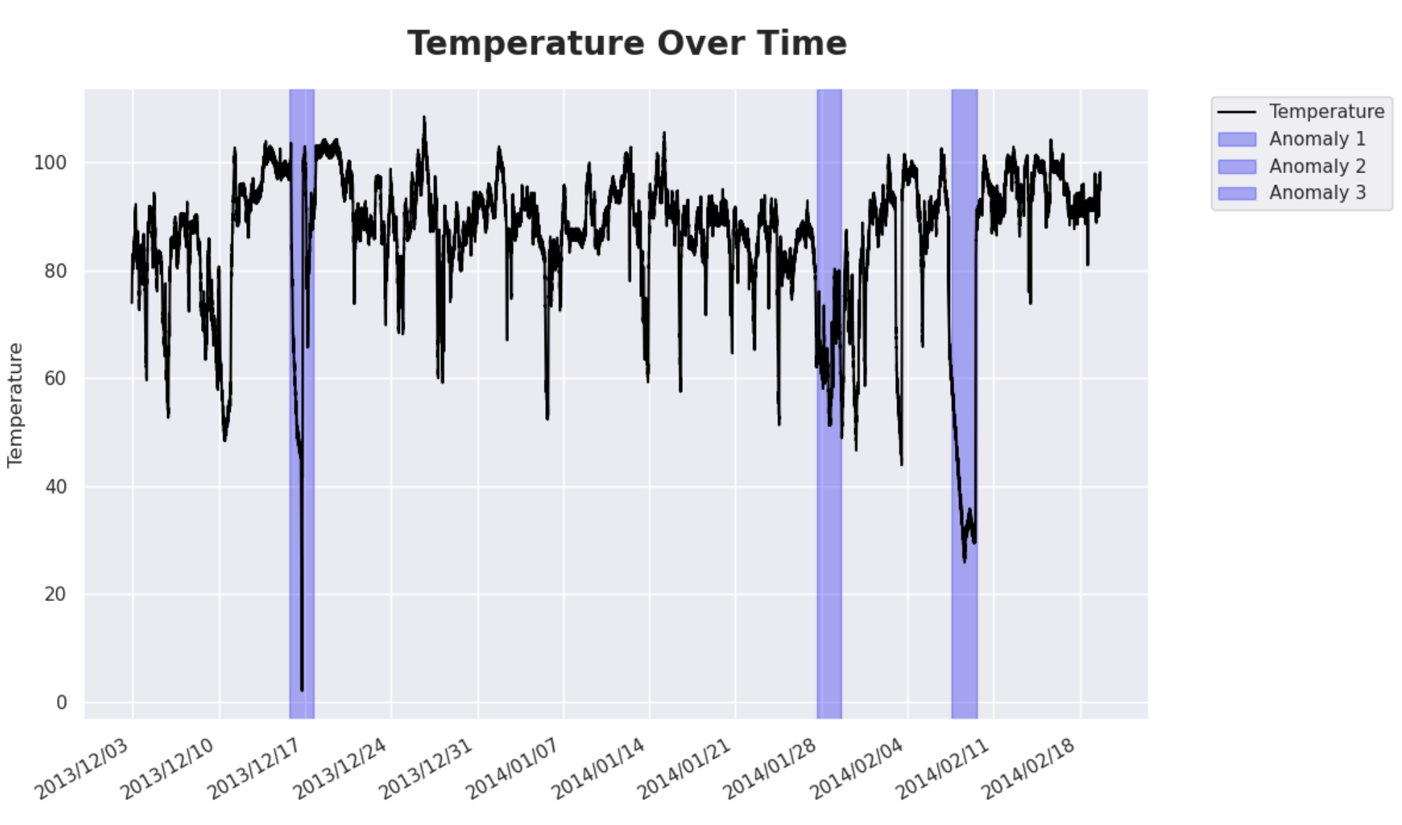
Observations on Time Series Data
Please note the blue highlighted areas above - these are real, observed anomalies in the dataset. You will use them later to evaluate the model. The first anomaly is a planned shutdown of the machine. The second anomaly is difficult to detect and directly led to the third anomaly, a catastrophic failure of the machine.
You see that there are some nasty spikes in the data, which make anomalies hard to differentiate from ordinary measurements. However, as you will see later, modern models are quite good at finding exactly those spots.
Model Training for Time Series Data
To get there, let's train a small anomaly detection model. As mentioned in the introduction, there are a multitude of options to choose from. This post will not go into the very details of model selection, and will just use the Merlion library, an excellent open-source time series analysis package developed by Salesforce.
Merlion implements an end-to-end machine learning framework, that includes loading and transforming data, building and training models, post-processing model outputs, and evaluating model performance. It supports various time series learning tasks, including forecasting, anomaly detection, and change point detection.
Start by first splitting the dataset into training and test data. The exercise will use unsupervised learning, so you want to train the model on data without anomalies, and then check whether it is able to detect the anomalies in the test data. The data will be split at 2013-12-15.
Now, train the model using the Merlion DefaultDetector, which is an anomaly detection model that balances performance and efficiency. Under the hood, the DefaultDetector is an ensemble of an ETS model and a Random Cut Forest model, both are excellent for general purpose anomaly detection.
Evaluation
Let's visually confirm the model performance:
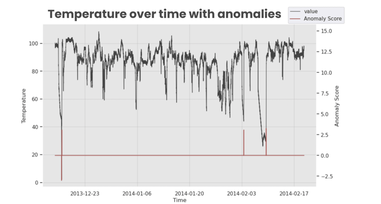
The model is able to detect the anomalies, a very good result for the first try, and without any parameter tuning. The next steps will bring this model to production.
In a real-world scenario, you want to further improve the model by tuning the parameters and evaluating the model performance on a validation dataset. However, for the sake of simplicity, this step will be skipped. Please refer to the Merlion documentation for more information on how to do this.
If you're excited about the potential of time-series data and want to optimize your MLOps workflow, then you won't want to miss Part 2 of this post series. We'll show you how CrateDB supports MLOps using the powerful mlflow python library. And, in Part 3, we'll take it a step further by demonstrating how CrateDB alone can support an entire MLOps lifecycle. Stay tuned for more!